Traveling Salesman Problem

The Traveling Salesman Problem (TSP) is the problem of finding the shortest tour for a salesman to visit every city exactly once and return to the starting point. In this tutorial, we explain how to solve the TSP using the metropolitan area of Japan as an example.

Mathematical model

In the following, we consider the TSP with \(n\) cities. Although several linear formulations for the TSP are known, in this tutorial we adopt the following quadratic formulation.

Decision variable

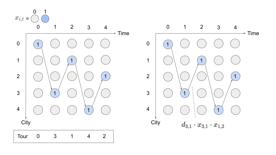
A binary variable \(x_{i,t}\) is defined as:

\[\begin{split} x_{i,t} = \begin{cases} 1~\text{if the salesman visits city }i\text{ at time }t\\ 0~\text{otherwise} \end{cases} \end{split}\]

\[ i, t \in \{0, ..., n-1\} \]

That is, \(x_{i, t}\) is 1 if the salesman visits city \(i\) at the \(t\)-th step, and 0 otherwise.

Constraints

We consider the following two constraints:

1. Each city is visited only once

\[ \sum_t x_{i, t} = 1, ~\forall i \]

2. Only one city is visited at each step

\[ \sum_i x_{i, t} = 1, ~\forall t \]

These two constraints are necessary for \(x_{i, t}\) to represent the order in which the salesman visits the cities. The salesman cannot visit multiple cities at the same time, nor does he need to visit the same city more than once.

The following figure illustrates an example assignment to \(x_{i, t}\) that satisfies these two constraints. This image will help you understand the formulation.

Objective function

Finally, let’s consider the objective function. The TSP aims to minimize the total travel distance, which can be formulated as follows:

\[ \sum_{i,j,t} d_{i, j}x_{i, t}x_{j, (t+1)\mod n} \]

Here, \(d_{i, j}\) is the distance between city \(i\) and city \(j\). \(x_{i, t}x_{j, t+1}\) is 1 if city \(i\) is visited at step \(t\) and city \(j\) at step \(t+1\), and 0 otherwise. The \(\mod n\) in \(x_{j, (t+1)\mod n}\) represents the return from the last city to the starting city.

\(n\)-city TSP

With these, the \(n\)-city TSP can be formulated as follows:

\[\begin{split} \begin{aligned} \min_x & \sum_{i, j, t} d_{i, j} x_{i,t} x_{j, (t+1) \mod n}\\ \mathrm{s.t.}~&\sum_i x_{i, t} = 1,~\forall t\\ &\sum_t x_{i, t} = 1, ~\forall i\\ &x_{i, t} \in \{0, 1\} \end{aligned} \end{split}\]

Modeling by JijModeling

We show an implementation using JijModeling. We first define the variables and parameters appearing in the mathematical model described above.

import jijmodeling as jm

problem = jm.Problem("TSP")
N = problem.Natural("N")
d = problem.Float("d", shape=(N, N))
x = problem.BinaryVar("x", shape=(N, N))

Here, N is the number of cities, and d is a two-dimensional list whose elements represent the distance \(d_{i, j}\) between city \(i\) and city \(j\). The binary variable x is defined to correspond to \(x_{i, t}\).

Implementing the objective function

Next, let’s set the objective function.

problem += jm.sum(
    jm.product(N, N, N),
    lambda i, j, t: d[i, j] * x[i, t] * x[j, (t + 1) % N],
)

Implementing the constraints

Then let’s define the two constraints.

problem += problem.Constraint(
    "one-city", lambda t: jm.sum(N, lambda i: x[i, t]) == 1, domain=N
)
problem += problem.Constraint(
    "one-time", lambda i: jm.sum(N, lambda t: x[i, t]) == 1, domain=N
)

Here, the constraint named "one-city" defines the constraint that only one city is visited at time \(t\). And the constraint named "one-time" sets the constraint that city \(i\) is visited only once.

This completes the implementation of the mathematical model. Let’s check that the mathematical model is correctly implemented through the LaTeX display.

problem

\[\begin{split}\begin{array}{rl} \text{Problem}\colon &\text{TSP}\\\displaystyle \min &\displaystyle \sum _{i=0}^{N-1}{\sum _{j=0}^{N-1}{\sum _{t=0}^{N-1}{{d}_{i,j}\cdot {x}_{i,t}\cdot {x}_{j,\left(t+1\right)\bmod N}}}}\\&\\\text{s.t.}&\\&\begin{aligned} \text{one-city}&\quad \displaystyle \sum _{i=0}^{N-1}{{x}_{i,t}}=1\quad \forall t\;\text{s.t.}\;t\in \left\{0,\ldots ,N-1\right\}\\\text{one-time}&\quad \displaystyle \sum _{t=0}^{N-1}{{x}_{i,t}}=1\quad \forall i\;\text{s.t.}\;i\in \left\{0,\ldots ,N-1\right\}\end{aligned} \\&\\\text{where}&\\&\text{Decision Variables:}\\&\qquad \begin{alignedat}{2}x&\in \mathop{\mathrm{Array}}\left[N\times N;\left\{0, 1\right\}\right]&\quad &2\text{-dim binary variable}\\\end{alignedat}\\&\\&\text{Placeholders:}\\&\qquad \begin{alignedat}{2}d&\in \mathop{\mathrm{Array}}\left[N\times N;\mathbb{R}\right]&\quad &2\text{-dimensional array of placeholders with elements in }\mathbb{R}\\N&\in \mathbb{N}&\quad &\text{A scalar placeholder in }\mathbb{N}\\\end{alignedat}\end{array} \end{split}\]

Prepare an instance

We prepare the number of cities and their coordinates. Here we select a metropolitan area in Japan.

import numpy as np

# set the name list of traveling points
points = ['Ibaraki', 'Tochigi', 'Gunma', 'Saitama', 'Chiba', 'Tokyo', 'Kanagawa']

# set the latitudes and longitudes of traveling points
latlng_list = [
    [36.2869536, 140.4703384],
    [36.6782167, 139.8096549],
    [36.52198, 139.033483],
    [35.9754168, 139.4160114],
    [35.549399, 140.2647303],
    [35.6768601, 139.7638947],
    [35.4342935, 139.374753]
]

# make distance matrix
inst_N = len(points)
inst_d = np.zeros((inst_N, inst_N))
for i in range(inst_N):
    for j in range(inst_N):
        a = np.array(latlng_list[i])
        b = np.array(latlng_list[j])
        inst_d[i][j] = np.linalg.norm(a-b)

# normalize distance matrix
inst_d = (inst_d-inst_d.min()) / (inst_d.max()-inst_d.min())

geo_data = {'points': points, 'latlng_list': latlng_list}
instance_data = {'N': inst_N, 'd': inst_d}

Solve by JijZeptSolver

We solve this problem using jijzept_solver.

import jijzept_solver

instance = problem.eval(instance_data)
solution = jijzept_solver.solve(instance, solve_limit_sec=1.0)

Visualize the solution

Let’s visualize the order in which the salesman visits the cities using the obtained solution.

import matplotlib.pyplot as plt

df = solution.decision_variables_df
x_indices = df[df["value"] == 1.0]["subscripts"]
tour = [index for index, _ in sorted(x_indices, key=lambda x: x[1])]
tour.append(tour[0])

position = np.array(geo_data['latlng_list']).T[[1, 0]]

plt.axes().set_aspect('equal')
plt.plot(*position, "o")
plt.plot(position[0][tour], position[1][tour], "-")
plt.show()

print(np.array(geo_data['points'])[tour])

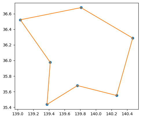
['Saitama' 'Gunma' 'Tochigi' 'Ibaraki' 'Chiba' 'Tokyo' 'Kanagawa'
 'Saitama']