
Minimum Maximal Matching#
We show how to solve the minimum maximal matching problem using JijZeptSolver and JijModeling. This problem is also mentioned in 4.5. Minimal Maximal Matching on Lucas, 2014, “Ising formulations of many NP problems”.
What is Minimum Maximal Matching?#
The minimum maximal matching problem is one of the matching problems in graphs. It asks for a set of edges in a graph such that no two selected edges share a vertex.
We assume that we have an undirected graph \(G = (V,E)\) and that \(C \subseteq E\) is a set of selected edges. The constraints on \(C\) are given as follows.
No two distinct edges in \(C\) share a vertex (matching condition).
Let \(D\) be the set of vertices connected to edges in \(C\). If \((u, v) \in E\), then it cannot be the case that \(u, v \in (V \setminus D)\) (maximality condition).
The second condition corresponds to maximality because, if \(u, v \in (V \setminus D)\), adding the edge \((u, v)\) to \(C\) would still preserve the matching condition.
The minimum maximal matching problem asks for a set of edges \(C\) that satisfies these two constraints and has the smallest possible number of edges.
Example#
For example, consider that we have a graph \(G = (V, E)\), where \(V = \{1,2,3,4,5\}\) and where \(E = \{(1,2),(1,3),(2,3),(3,4),(4,5)\}\). To find a maximal matching, we first have the empty set as a matching. Then, we add edges to the matching until we cannot add any more edges without violating the matching condition.
In such a small problem, one may be able to find the minimum maximal matching with some trial and error. In this case, the answer is \(\{(1, 2), (3, 4)\}\) or \(\{(1, 3), (4, 5)\}\), \(\{(2, 3), (4, 5)\}\).
Mathematical model#
A binary variable \(x_e\) denotes whether or not the edge \(e\) is colored; the edge is colored if \(x_e\) is 1, and vice versa. We also introduce a binary variable \(y_v\) that denotes whether or not the vertex \(v\) is included in the matching (\(D\) in the above statements); the vertex is connected to an edge in \(C\) if \(y_v = 1\), and vice versa.
Constraint 1: relationship between \(x\) and \(y\)
Let \(E_v\) be the set of edges incident to vertex \(v\).
By the definitions of the two binary variables \(x\) and \(y\), \(y_v = 1\) is equivalent to \(\sum_{e \in E_v} x_e \ge 1\). Since the first condition (the matching condition) requires \(\sum_{e \in E_v} x_e \le 1\), we can write the following equality:
Constraint 2: Every unselected edge is connected to at least one vertex connected to a selected edge
To formulate this maximality constraint, we use a basic observation: \(1-y_u\) is 0 if \(u\) is connected to a selected edge, and vice versa. Then, by counting \((1-y_{u})(1-y_{v})\) for all \((u,v) \in E\), we can check the violation of the constraint; i.e. if \((1-y_{u})(1-y_{v}) > 0\) for any \((u,v) \in E\), the edge \((u,v)\) can be selected without violating the constraints. $\( \quad \sum_{(u,v)\in E} (1-y_u)(1-y_v) = 0. \)$
Objective function: minimize the size of the matching
The size here means the number of edges selected. $\( \quad \min \sum_{e \in E} x_e. \)$
Modeling by JijModeling#
Next, we show how to implement the above equations using JijModeling. We first define the variables in the mathematical model described above.
import jijmodeling as jm

# define problem
problem = jm.Problem('Minimum Maximal Matching')

# define variables
V = problem.Natural('V')
E = problem.Graph('E', dtype=V)
num_E = problem.NamedExpr('num_E', E.len_at(0))
x = problem.BinaryVar('x', shape=(num_E,))
y = problem.BinaryVar('y', shape=(V,))
Constraints and objective function#
The constraints and the objective function are written as:
problem += problem.Constraint(
    'y_x_relation',
    lambda v: y[v] - jm.sum(jm.filter(lambda e: (E[e][0]==v)|(E[e][1]==v), num_E), lambda e: x[e]) == 0,
    domain=V
)
problem += problem.Constraint(
    'unselected_edge',
    jm.sum(num_E, lambda e: (1-y[E[e][0]])*(1-y[E[e][1]]))==0
)

problem += x.sum()
On Jupyter Notebook, one can check the problem statement in a human-readable way by evaluating the following cell.
problem
Prepare an instance#
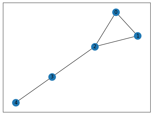
Here we use the same instance with an example described above.
import networkx as nx

# set empty graph
inst_G = nx.Graph()
V = [0, 1, 2, 3, 4]
# add edges
inst_E = [[0, 1], [0, 2], [1, 2], [2, 3], [3, 4]]
inst_G.add_edges_from(inst_E)
# get the number of nodes
inst_V = list(inst_G.nodes)
num_V = len(inst_V)
instance_data = {'V': num_V, 'E': inst_E}
This graph is shown below.
import matplotlib.pyplot as plt

pos = nx.spring_layout(inst_G)
nx.draw_networkx(inst_G, pos=pos, with_labels=True)
plt.show()
Solve by JijZeptSolver#
We solve this problem using jijzept_solver.
import jijzept_solver

instance = problem.eval(instance_data)
solution = jijzept_solver.solve(instance, solve_limit_sec=1.0)
Visualize the solution#
The optimized solution can be seen as below.
import numpy as np

# get the indices of x == 1
df = solution.decision_variables_df
x_indices = np.ravel(df[(df["name"] == "x") & (df["value"] == 1.0)]["subscripts"].to_list())
# get the indices of y == 1
y_indices = np.ravel(df[(df["name"] == "y") & (df["value"] == 1.0)]["subscripts"].to_list())
# set color list for visualization
cmap = plt.get_cmap("tab10")
# set vertex color
vertex_colors = [cmap(1) if i in y_indices else cmap(0) for i in inst_V]
# set edge color list
edge_colors = ["red" if j in x_indices else "black" for j, _ in enumerate(instance_data["E"])]
# dwaw the figure with two subplots
fig, (ax1, ax2) = plt.subplots(1, 2, figsize=(10, 5))
# plot the initial graph
nx.draw_networkx(inst_G, pos, with_labels=True, ax=ax1)
ax1.set_title('Initial Graph')
plt.axis('off')
ax1.set_frame_on(False) # Remove the frame from the first subplot
# plot the minimum maximal matching graph
nx.draw_networkx(inst_G, pos=pos, node_color=vertex_colors, edge_color=edge_colors, with_labels=True)
plt.axis('off')
ax2.set_title('Minimum Maximal Matching Graph')
# Show the plot
plt.show()
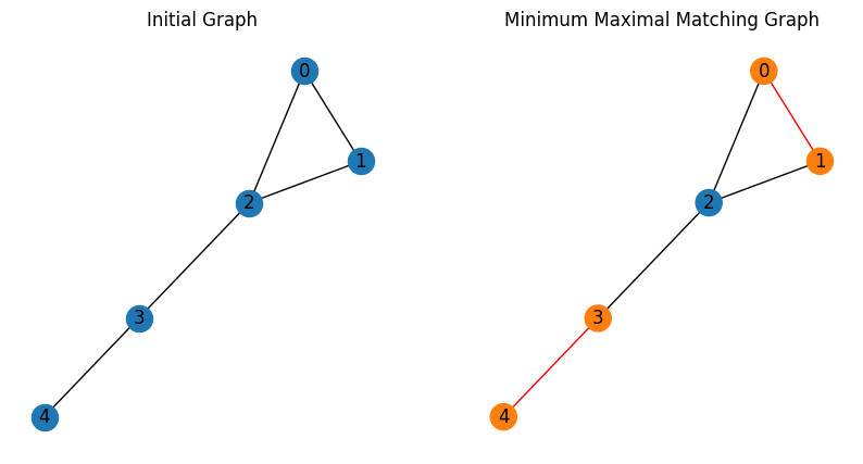
As expected, we have obtained the minimum maximal matching graph.