Item Listing Optimization for E-Commerce Websites Based on Diversity#
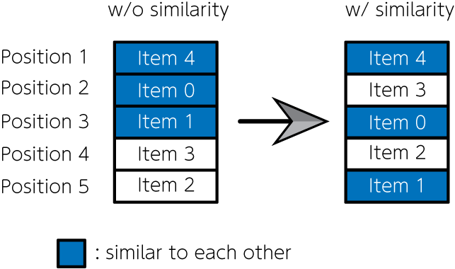
E-commerce sites with billing systems, such as product sales, hotel reservations, and music and video streaming sites, have become familiar to us today. These sites list a wide variety of items. One of the most important issues on these websites is how to decide which items to list and how to arrange them. That problem directly affects sales on e-commerce sites. If items are simply ordered by popularity (e.g., number of sales), highly similar items are often placed consecutively, which may lead to a bias toward a specific preference. Therefore, Nishimura et al. (2019) formulated the item listing problem as a quadratic assignment problem, using penalties for items with high similarity being placed next to each other. They then solved the problem with quantum annealing and succeeded in creating an item list that simultaneously accounts for item popularity and diversity. In this article, we implement the mathematical model using JijModeling and solve it using JijZeptSolver.
A mathematical model#
Let us consider which items are listed in which positions on a given website. We define the set of items to be listed as \(I\) and the set of positions where items are listed as \(J\). We use a binary variable \(x_{i, j} = 1\) that represents assigning item \(i\) to position \(j\), and \(x_{i, j} = 0\) otherwise.
Ensure that each item is allocated to exactly one position#
Ensure that each position is allocated exactly one item#
An objective function#
\(s_{ij}\) is the estimated sales of an item \(i \in I\) when it is placed in a position \(j \in J\), then total estimated sales for all items is
However, as mentioned above, the objective function (3) leads to a result in listing only items of the same preference, obtaining a solution that cannot be considered an optimal arrangement. Therefore, we introduce the following term in the objective function.
where \(f_{ii'}\) is the items’ similarity degree between item \(i\) and \(i'\), and \(d_{jj'}\) is the adjacent flag of the position \(j\) and \(j'\); \(d_{jj'} = 1\) is for the adjacent positions, otherwise \(d_{jj'} =0\). By introducing this term into the above objective function, we can get results in which items with small similarity are lined up in adjacent positions. From the above discussion, the function we have to maximize in this optimization problem is expressed as follows:
where \(w\) represents a weight of second term.
Decomposition Methods for Item Listing Problem#
For large problems, a feasible solution may not be found, or a feasible solution may be far from optimal. Therefore, we first solve the optimization problem with equation (3) as the objective function. Then, we solve the problem using equation (5) for the upper positions of the item list. This scheme effectively determines the items that are browsed most often.
Modeling by JijModeling#
Let’s implement a script for solving this problem using JijModeling and JijZeptSolver.
Defining variables#
We define the variables to be used for optimization. First, we consider the implementation of the mathematical model using equation (3) as the objective function.
import jijmodeling as jm

# make problem
problem = jm.Problem('E-commerce', sense=jm.ProblemSense.MAXIMIZE)

# define variables
I = problem.Natural('I')
J = problem.Natural('J')
s = problem.Float('s', shape=(I, J))
x = problem.BinaryVar('x', shape=(I, J))
where I is the set of items, J is the set of positions, s is the matrix representing the estimated sales, and x is the binary variable. Note that we set jm.Problem(..., sense=jm.ProblemSense.MAXIMIZE) since this is a maximization problem.
Implementation for E-commerce optimization#
Then, we implement the mathematical model represented by the constraints in equations (1) and (2), and the objective function in equation (3).
# set constraint 1: onehot constraint for items
problem += problem.Constraint('onehot-items', lambda i: jm.sum(J, lambda j: x[i, j])==1, domain=I)
# set constraint 2: onehot constraint for position
problem += problem.Constraint('onehot-positions', lambda j: jm.sum(I, lambda i: x[i, j])==1, domain=J)
# set objective function 1: maximize the sales
problem += jm.sum(jm.product(I, J), lambda i, j: s[i, j] * x[i, j])
Let’s check the mathematical model we’ve created so far.
problem
Creating an instance#
Next, we create instances corresponding to I, J, and s.
Here we set that the number of items is 10, and the number of positions where the items are listed is also 10.
In addition, the estimated sales matrix s is assumed to be random.
import numpy as np

np.random.seed(seed=0)

# set the number of items
inst_I = 10
inst_J = 10
inst_s = np.random.rand(inst_I, inst_J)
instance_data = {'I': inst_I, 'J': inst_J, 's': inst_s}
Solve by JijZeptSolver#
We solve this problem using jijzept_solver.
import jijzept_solver

instance = problem.eval(instance_data)
solution = jijzept_solver.solve(instance, solve_limit_sec=1.0)
Check the solution#
Let’s check the solution obtained.
df = solution.decision_variables_df
x_indices = np.array(df[df["value"]==1]["subscripts"].to_list())
# initialize binary array
pre_binaries = np.zeros([inst_I, inst_J], dtype=int)
# input solution into array
pre_binaries[x_indices[:, 0], x_indices[:, 1]] = 1
# format solution for visualization
pre_zip_sort = sorted(zip(np.where(np.array(pre_binaries))[1], np.where(np.array(pre_binaries))[0]))
for pos, item in pre_zip_sort:
    print('{}: item {}'.format(pos, item))
0: item 0
1: item 3
2: item 7
3: item 5
4: item 4
5: item 6
6: item 9
7: item 2
8: item 1
9: item 8
Decomposition: Leveraging penalty term and fixed variables#
Next, we further solve the problem with the objective function in equation (5), which takes into account item similarity for the top positions. To this purpose, we define new variables.
# set variables for sub-problem
f = problem.Float('f', shape=(I, I))
d = problem.Float('d', shape=(J, J))
fixed_IJ = problem.Placeholder('fixed_IJ', dtype=(I, J), ndim=1)
num_fixed_IJ = problem.NamedExpr("num_fixed_IJ", fixed_IJ.len_at(0))
w = problem.Float('w')
fixed_IJ represents the set of indices that fix the variables, which means they are not solved in the next execution (i.e., corresponding to items appearing in lower positions and their positions).
This is expressed as a two-dimensional array, e.g., fixed_IJ = [[5, 6], [7, 8]] represents \(x_{5, 6} = 1, x_{7, 8} = 1\).
f is the item similarity matrix, d is the adjacent flag matrix.
Next, we add a term to minimize the sum of the similarities.
# set penalty term 2: minimize similarity
problem += - w * jm.sum(jm.product(I, I, J, J), lambda i1, i2, j1, j2: f[i1, i2] * d[j1, j2] * x[i1, j1] * x[i2, j2])
Finally, we add a constraint to fix the variables for items appearing in lower positions.
# set fixed variables
problem += problem.Constraint('fix', lambda v: x[fixed_IJ[v][0], fixed_IJ[v][1]]==1, domain=num_fixed_IJ)
We can describe fixing variables as a trivial constraint via Constraint.
Let’s display the newly added terms and constraints.
problem
Now that we’ve finished implementing the mathematical model, let’s create instances for item similarity and fixed variables.
# set instance for similarity term
inst_f = np.random.rand(inst_I, inst_I)
triu = np.tri(inst_J, k=1) - np.tri(inst_J, k=0)
inst_d = triu + triu.T
# set instance for fixed variables
reopt_N = 5
item_indices = x_indices[:, 0]
position_indices = x_indices[:, 1]
fixed_indices = np.where(np.array(position_indices)>=reopt_N)
fixed_items = np.array(item_indices)[fixed_indices]
fixed_positions = np.array(position_indices)[fixed_indices]
inst_fixed_IJ = np.array([[x, y] for x, y in zip(fixed_items, fixed_positions)])
# set weight fo the penalty
inst_w = 1.0

instance_data = {'I': inst_I, 'J': inst_J, 's': inst_s, 'f': inst_f, 'd': inst_d, 'fixed_IJ': inst_fixed_IJ, 'w': inst_w}
Then, let’s solve the mathematical model considering the similarity penalty and fixed variables with JijZeptSolver.
instance = problem.eval(instance_data)
solution = jijzept_solver.solve(instance, solve_limit_sec=1.0)
Again, let’s check the solution obtained.
df = solution.decision_variables_df
x_indices = np.array(df[df["value"]==1]["subscripts"].to_list())
# initialize binary array
post_binaries = np.zeros([inst_I, inst_J], dtype=int)
# input solution into array
post_binaries[x_indices[:, 0], x_indices[:, 1]] = 1
# format solution for visualization
post_zip_sort= sorted(zip(np.where(np.array(post_binaries))[1], np.where(np.array(post_binaries))[0]))
for i, j in post_zip_sort:
    print('{}: item {}'.format(i, j))
0: item 0
1: item 3
2: item 7
3: item 5
4: item 4
5: item 6
6: item 9
7: item 2
8: item 1
9: item 8
Let us compare these two results.
items = ["Item {}".format(i) for i in np.where(pre_binaries==1)[0]]
pre_order = np.where(pre_binaries==1)[1]
post_order = np.where(post_binaries==1)[1]
To plot a graph, we define the following class.
from typing import Optional
import matplotlib.pyplot as plt

class Slope:
    """Class for a slope chart"""
    def __init__(self,
        figsize: tuple[float, float] = (6,4),
        dpi: int = 150,
        layout: str = 'tight',
        show: bool =True,
        **kwagrs):

        self.fig = plt.figure(figsize=figsize, dpi=dpi, layout=layout, **kwagrs)
        self.show = show

        self._xstart: float = 0.2
        self._xend: float = 0.8
        self._suffix: str = ''
        self._highlight: dict = {}

    def __enter__(self):
        return(self)

    def __exit__(self, exc_type, exc_value, exc_traceback):
        plt.show() if self.show else None

    def highlight(self, add_highlight: dict) -> None:
        """Set highlight dict

        e.g.
            {'Group A': 'orange', 'Group B': 'blue'}

        """
        self._highlight.update(add_highlight)

    def config(self, xstart: float =0, xend: float =0, suffix: str ='') -> None:
        """Config some parameters

            Args:
                xstart (float): x start point, which can take 0.0〜1.0
                xend (float): x end point, which can take 0.0〜1.0
                suffix (str): Suffix for the numbers of chart e.g. '%'

            Return:
                None

        """
        self._xstart = xstart if xstart else self._xstart
        self._xend = xend if xend else self._xend
        self._suffix = suffix if suffix else self._suffix

    def plot(self, time0: list[float], time1: list[float],
             names: list[float], xticks: Optional[tuple[str,str]] = None,
             title: str ='', subtitle: str ='', ):
        """Plot a slope chart

        Args:
            time0 (list[float]): Values of start period
            time1 (list[float]): Values of end period
            names (list[str]): Names of each items
            xticks (tuple[str, str]): xticks, default to 'Before' and 'After'
            title (str): Title of the chart
            subtitle (str): Subtitle of the chart, it might be x labels

        Return:
            None

        """

        xticks = xticks if xticks else ('Before', 'After')

        xmin, xmax = 0, 4
        xstart = xmax * self._xstart
        xend = xmax * self._xend
        ymax = max(*time0, *time1)
        ymin = min(*time0, *time1)
        ytop = ymax * 1.2
        ybottom = ymin - (ymax * 0.2)
        yticks_position = ymin - (ymax * 0.1)

        text_args = {'verticalalignment':'center', 'fontdict':{'size':10}}

        for t0, t1, name in zip(time0, time1, names):
            color = self._highlight.get(name, 'gray') if self._highlight else None

            left_text = f'{name} {str(round(t0))}{self._suffix}'
            right_text = f'{str(round(t1))}{self._suffix}'

            plt.plot([xstart, xend], [t0, t1], lw=2, color=color, marker='o', markersize=5)
            plt.text(xstart-0.1, t0, left_text, horizontalalignment='right', **text_args)
            plt.text(xend+0.1, t1, right_text, horizontalalignment='left', **text_args)

        plt.xlim(xmin, xmax)
        plt.ylim(ytop, ybottom)

        plt.text(0, ytop, title, horizontalalignment='left', fontdict={'size':15})
        plt.text(0, ytop*0.95, subtitle, horizontalalignment='left', fontdict={'size':10})

        plt.text(xstart, yticks_position, xticks[0], horizontalalignment='center', **text_args)
        plt.text(xend, yticks_position, xticks[1], horizontalalignment='center', **text_args)
        plt.axis('off')


def slope(
    figsize=(6,4),
    dpi: int = 150,
    layout: str = 'tight',
    show: bool =True,
    **kwargs
    ):
    """Context manager for a slope chart"""

    slp = Slope(figsize=figsize, dpi=dpi, layout=layout, show=show, **kwargs)

    return slp
Finally, let’s display a graph for comparison.
# compute similarity for the first
A = np.dot(instance_data['f'], pre_binaries)
B = np.dot(pre_binaries, instance_data['d'])
AB = A * B
pre_similarity = np.sum(AB)

# compute similarity for the second
A = np.dot(instance_data['f'], post_binaries)
B = np.dot(post_binaries, instance_data['d'])
AB = A * B
post_similarity = np.sum(AB)

pre_string = "Similarity: {:.2g}".format(pre_similarity)
post_string = "Similarity: {:.2g}".format(post_similarity)
with slope() as slp:
    slp.plot(pre_order, post_order, items, (pre_string, post_string))
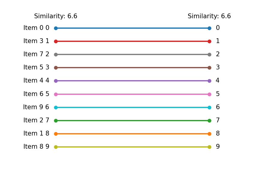
Compared to the first optimization results, the lower part shows no change due to the fixed variables. However, in the upper part, changes in order can be observed due to considering similarity.