
Vertex Cover Problem#
We show how to solve the vertex cover problem using JijZeptSolver and JijModeling. This problem is also mentioned in 4.3. Vertex Cover on Lucas, 2014, “Ising formulations of many NP problems”.
What is the Vertex Cover Problem?#
Given an undirected graph \(G = (V, E)\), the vertex cover problem asks for a smallest set \(V' \subseteq V\) that covers the edge set \(E\). Here, a set of vertices \(V'\) covers the edge set \(E\) if, for every edge \(e \in E\), at least one endpoint of \(e\) is an element of \(V'\).
For example, consider the following undirected graph:
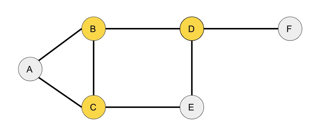
This graph has vertices \(A, B, C, D, E, F\) and seven edges connecting them.
Now consider the vertex set \(V' := \{B, C, D\}\). This set covers the edge set because:
For edge \((A, B)\), \(B \in V'\)
For edge \((A, C)\), \(C \in V'\)
For edge \((B, C)\), \(B \in V'\)
For edge \((B, D)\), \(B \in V'\)
For edge \((C, E)\), \(C \in V'\)
For edge \((D, E)\), \(D \in V'\)
For edge \((D, F)\), \(D \in V'\)
Mathematical model#
First, we introduce binary variables \(x_{v}\) that take 1 if vertex \(v\) is selected and take 0 otherwise.
Constraint: every edge has at least one selected endpoint#
For every edge \((u, v)\), vertex \(u\), vertex \(v\), or both must be included in the vertex cover.
Objective function: minimize the size of the vertex cover#
This can be expressed as follows: $\( \quad \min \sum_v x_v. \)$
Modeling by JijModeling#
Next, we show how to implement the above equations using JijModeling. We first define the variables in the mathematical model described above. (Cf. graph partitioning problem.)
import jijmodeling as jm

problem = jm.Problem('Vertex Cover')

V = problem.Natural('V')
E = problem.Graph('E', dtype=V)
x = problem.BinaryVar('x', shape=(V,))
Constraint and objective function#
The constraint and the objective function are written as:
problem += jm.sum(V, lambda v: x[v])
problem += problem.Constraint('color', jm.sum(E, lambda e: (1-x[e[0]])*(1-x[e[1]])) == 0)
On Jupyter Notebook, one can check the problem statement in a human-readable way by evaluating the following cell.
problem
Prepare an instance#
We prepare a graph using Networkx.
import networkx as nx

# set the number of vertices
inst_V = 12
# create a random graph
inst_G = nx.gnp_random_graph(inst_V, 0.4)
# get information of edges
inst_E = [list(edge) for edge in inst_G.edges]
instance_data = {'V': inst_V, 'E': inst_E}
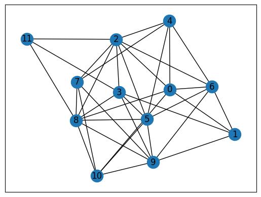
This graph is shown below.
import matplotlib.pyplot as plt

nx.draw_networkx(inst_G, with_labels=True)
plt.show()
Solve by JijZeptSolver#
We solve this problem using jijzept_solver.
import jijzept_solver

instance = problem.eval(instance_data)
solution = jijzept_solver.solve(instance, solve_limit_sec=1.0)
Visualize solution#
Finally, we visualize the solution obtained.
import matplotlib.pyplot as plt
import numpy as np

# get the indices of x == 1
df = solution.decision_variables_df
x_indices = np.ravel(df[df["value"]==1]["subscripts"].to_list())
# set color list for visualization
cmap = plt.get_cmap("tab10")
# initialize vertex color list
node_colors = [cmap(0)] * instance_data["V"]
# set vertex color list
for i in x_indices:
    node_colors[i] = cmap(1)
# draw the graph
nx.draw_networkx(inst_G, node_color=node_colors, with_labels=True)
plt.show()
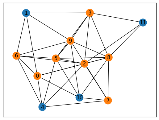
The above figure clearly shows a feasible vertex cover for the given graph.