Minimum Spanning Tree with a Maximum Degree Constraint

We show how to solve the minimum spanning tree problem with a maximum degree constraint using JijZeptSolver and JijModeling. This problem is also mentioned in 8.1. Minimal Spanning Tree with a Maximal Degree Constraint on Lucas, 2014, “Ising formulations of many NP problems”.

What is Minimum Spanning Tree with a Maximum Degree Constraint?

The minimum spanning tree problem is defined as follows. Given an undirected graph \(G = (V, E)\), where each edge \((uv) \in E\) is associated with a cost \(c_{uv}\), construct the spanning tree (a tree that contains all vertices) \(T \subseteq G\) such that the cost of \(T\)

\[ c(T) = \sum_{(uv) \in E_T} c_{uv} \]

is minimized if such a tree exists. One can add a degree constraint that forces each degree of a vertex in \(T\) to be \(\leq \Delta\).

Example

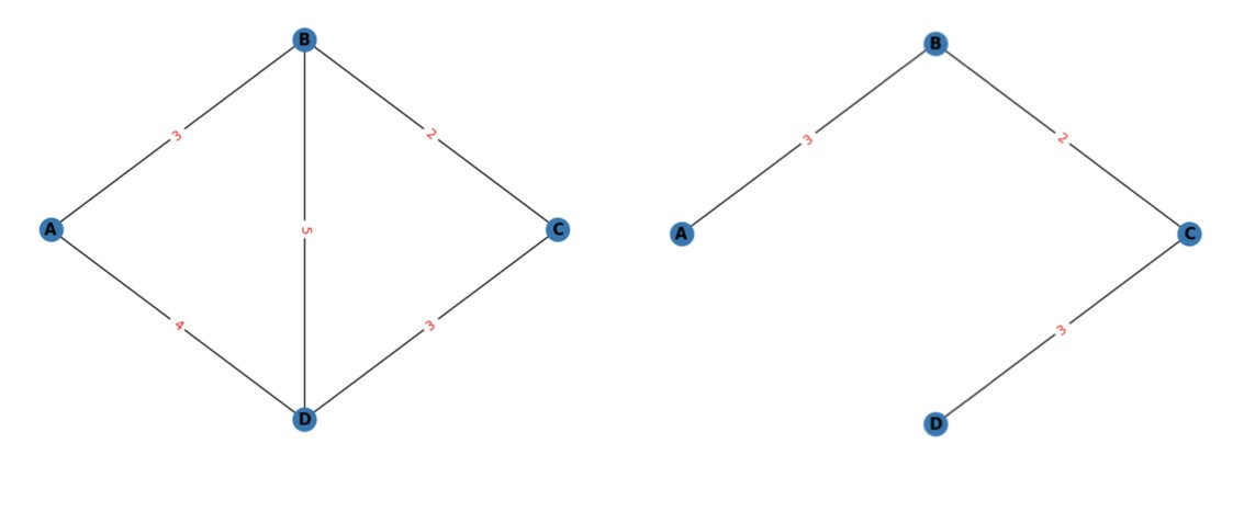
Let us consider a simple graph shown below. Suppose we want to find the minimum spanning tree of the left graph subject to a maximum degree constraint of 3. The solution to this problem is given on the right; the edges in this tree have a total weight of 8, which is the minimum possible, and the maximum degree constraint is satisfied.

Mathematical model

We first place a binary variable \(x_{uv}\) on each edge to show whether or not the edge is included in \(T\);

Constraint1: Each vertex can have at most \(\Delta\) edges

The degree of any vertex in the graph cannot exceed \(\Delta\). Note that we also have a lower bound condition for the degree of each vertex, because, in a spanning tree, each vertex must have at least one edge.

\[ \quad 1 \leq \sum_{(uv),(vu) \in E} x_{uv} \leq \Delta \quad \forall u \in V. \]

Note that the notation in the summation is meant to include both \(x_{uv}\) and \(x_{vu}\).

Constraint 2: The number of selected edges is \(|V|-1\)

The selected edge set must form a tree that contains all \(|V|\) vertices. Such a spanning tree has \(|V|-1\) edges.

\[ \quad \sum_{(uv) \in E} x_{uv} = |V|-1. \]

Constraint3: Absence of cycles

If \(T\) has a cycle \((v_1, v_2, \dots, v_k, v_1)\), then that cycle forms a connected subgraph of \(G\). Thus, if we consider the subgraph \(S\) induced by the vertices \(\{v_1, v_2, \dots, v_k\}\), the total number of selected edges inside \(S\) is greater than \(k-1\).

To eliminate such cases, we add a constraint requiring that, for every connected subgraph \(S\) of \(G\), the total number of selected edges inside \(S\) is at most \(|S|-1\).

\[ \quad \sum_{(uv) \in E(S)} x_{uv} \leq |S| - 1, \quad \forall (\text{connected } S) \subseteq G, \]

where \(E(S)\) represents the set of edges contained in \(S\). Together with Constraint 2, this constraint guarantees that the selected edge set has no cycles.

In general, for a spanning subgraph \(G'\) whose vertex set is \(V\) and that has \(|V|-1\) edges, the following are all equivalent: \(G'\) has no cycles, \(G'\) is connected, and \(G'\) is a spanning tree. Therefore, Constraints 2 and 3 guarantee that the selected edge set forms a spanning tree.

Objective function

We set the objective function so that the total weight of \(T\) is minimized.

\[ \quad \min \sum_{uv \in E} c_{uv}x_{uv}. \]

Modeling by JijModeling

Next, we show how to implement the above equations using JijModeling. We first define the variables in the mathematical model described above.

import jijmodeling as jm

# define problem
problem = jm.Problem("minimum spanning tree with a maximum degree constraint")

# define variables
V = problem.Natural('V')  # number of vertices
E = problem.Graph('E', dtype=V)  # set of edges
num_E = problem.NamedExpr('num_E', E.len_at(0))
C = problem.Float('C', dict_keys=E)  # cost of each edge
D = problem.Natural('D')  # maximum allowed degrees

# Each entry S[i] represents a connected subgraph and shall contain
# a list of (indices) of edges included in the subgraph, that is,
# if an edge E[k] is included in the subgraph represented by S[i], then k should be in S[i].
S = problem.Placeholder('S', dtype=num_E, shape=(None, num_E), jagged=True)
num_S = problem.NamedExpr('num_S', S.len_at(0))

# S_nodes[i] is the number of vertices in the subgraph represented by S[i].
S_nodes = problem.Natural('S_nodes', less_than=V, shape=(num_S,))

x = problem.BinaryVar('x', dict_keys=E)

The constraints and the objective function are written as:

problem += problem.Constraint(
    'const1-1',
    lambda v: jm.filter(lambda e: (e[0]==v)|(e[1]==v), E).map(lambda e: x[e]).sum() >= 1,
    domain=V
)
problem += problem.Constraint(
    'const1-2',
    lambda v: jm.filter(lambda e: (e[0]==v)|(e[1]==v), E).map(lambda e: x[e]).sum() <= D,
    domain=V
)
problem += problem.Constraint('const2', jm.sum(E, lambda e: x[e]) == V-1)
problem += problem.Constraint(
    'const3',
    lambda s: jm.sum(S[s], lambda e_i: x[E[e_i]]) <= S_nodes[s] - 1,
    domain=num_S
)
problem += jm.sum(E, lambda e: C[e] * x[e])

On Jupyter Notebook, one can check the problem statement in a human-readable way by evaluating the following cell.

problem

\[\begin{array}{rl} \text{Problem}\colon &\text{minimum spanning tree with a maximum degree constraint}\\\displaystyle \min &\displaystyle \sum _{e=0}^{num\_{}E-1}{{C}_{{E}_{e,0},{E}_{e,1}}\cdot {x}_{e}}\\&\\\text{s.t.}&\\&\begin{aligned} \text{const1-1}&\quad \displaystyle \sum _{\substack{e=0\\{E}_{e,0}=v\lor {E}_{e,1}=v}}^{num\_{}E-1}{{x}_{e}}\geq 1\quad \forall v\;\text{s.t.}\;v\in \left\{0,\ldots ,V-1\right\}\\\text{const1-2}&\quad \displaystyle \sum _{\substack{e=0\\{E}_{e,0}=v\lor {E}_{e,1}=v}}^{num\_{}E-1}{{x}_{e}}\leq D\quad \forall v\;\text{s.t.}\;v\in \left\{0,\ldots ,V-1\right\}\\\text{const2}&\quad \displaystyle \sum _{\vec{\imath }}{{{\left(x\right)}}_{\vec{\imath }}}=V-1\\\text{const3}&\quad \displaystyle \sum _{e\_{}s=0}^{\mathop{\mathtt{len\_{}at}}\left({S}_{i\_{}s},0\right)-1}{{x}_{e\_{}s}}\leq {S\_{}nodes}_{i\_{}s}-1\quad \forall i\_{}s\;\text{s.t.}\;i\_{}s\in \left\{0,\ldots ,num\_{}S-1\right\}\end{aligned} \\&\\\text{where}&\\&\text{Decision Variables:}\\&\qquad \begin{alignedat}{2}x&\in \mathop{\mathrm{Array}}\left[num\_{}E;\left\{0, 1\right\}\right]&\quad &1\text{-dim binary variable}\\\end{alignedat}\\&\\&\text{Placeholders:}\\&\qquad \begin{alignedat}{2}C&\in \mathop{\mathrm{Array}}\left[V\times V;\mathbb{R}\right]&\quad &2\text{-dimensional array of placeholders with elements in }\mathbb{R}\\D&\in \mathbb{N}&\quad &\text{A scalar placeholder in }\mathbb{N}\\E&\in \mathop{\mathrm{Array}}\left[(-);\mathbb{N}\times \mathbb{N}\right]&\quad &1\text{-dimensional array of placeholders with elements in }\mathbb{N}\times \mathbb{N}\\S&\in \mathop{\mathrm{JaggedArray}}\left[(-)\times (-)\times (-);\mathbb{R}\right]&\quad &3\text{-dimensional array of placeholders with elements in }\mathbb{R}\\S\_{}nodes&\in \mathop{\mathrm{Array}}\left[num\_{}S;\mathbb{N}\right]&\quad &1\text{-dimensional array of placeholders with elements in }\mathbb{N}\\V&\in \mathbb{N}&\quad &\text{A scalar placeholder in }\mathbb{N}\\\end{alignedat}\\&\\&\text{Named Expressions:}\\&\qquad \begin{alignedat}{2}num\_{}E&=\mathop{\mathtt{len\_{}at}}\left(E,0\right)&\quad &\in \mathbb{N}\\&&&\\num\_{}S&=\mathop{\mathtt{len\_{}at}}\left(S,0\right)&\quad &\in \mathbb{N}\\\end{alignedat}\end{array} \]

Prepare an instance

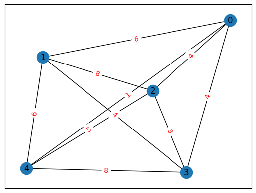
We prepare a graph using NetworkX. As an example, we create a random connected graph.

import itertools
import networkx as nx
import numpy as np

np.random.seed(seed=0)

# set the number of vertices
inst_V = 5
# set the number of degree
inst_D = 2

# set the probability of rewiring edges
p_rewire = 0.2
# set the number of nearest neighbors
k_neighbors = 4
# create a connected graph
inst_G = nx.connected_watts_strogatz_graph(inst_V, k_neighbors, p_rewire)
# add random costs to the edges
for u, v in inst_G.edges():
    inst_G[u][v]['weight'] = np.random.randint(1, 10)

# create a list of edges
inst_E = [tuple(edge) for edge in inst_G.edges()]

# create a dictionary for the costs
inst_C = {(u, v): inst_G[u][v]['weight'] for u, v in inst_E}

# get subgraphs and their edges
subs_nodes = []
subs_edges = []
# get connected subgraphs that have at least 2 nodes and have less nodes than the original graph
for num_nodes in range(2, inst_G.number_of_nodes()):
    for comb in (inst_G.subgraph(selected_nodes) for selected_nodes in itertools.combinations(inst_G, num_nodes)):
        if nx.is_connected(comb):
            edges_indices = [inst_E.index((u, v)) for u, v in comb.edges()]
            
            subs_edges.append(edges_indices)
            subs_nodes.append(comb.nodes)

inst_S = subs_edges
inst_S_nodes = [len(subgraph_nodes) for subgraph_nodes in subs_nodes]

instance_data = {'V': inst_V, 'D': inst_D, 'E': inst_E, 'C': inst_C, 'S': inst_S, 'S_nodes': inst_S_nodes}

This graph is shown below.

import matplotlib.pyplot as plt

pos = nx.spring_layout(inst_G)
nx.draw_networkx(inst_G, pos, with_labels=True)
edge_labels = nx.get_edge_attributes(inst_G, 'weight')
nx.draw_networkx_edge_labels(inst_G, pos, edge_labels=edge_labels, font_color='red')

plt.show()

Solve by JijZeptSolver

We solve this problem using jijzept_solver.

import jijzept_solver

instance = problem.eval(instance_data)
solution = jijzept_solver.solve(instance, solve_limit_sec=1.0)

Visualize the solution

The optimized solution can be seen as below.

# get the indices of x == 1
df = solution.decision_variables_df
x_indices = df[df["value"]==1]["subscripts"].to_list()

# draw figure
plt.subplot(121)
plt.axis('off')
nx.draw(inst_G, pos, with_labels=True, font_weight='bold')
nx.draw_networkx_edge_labels(inst_G, pos, edge_labels=edge_labels, font_color='red')
plt.subplot(122)
plt.axis('off')

inst_H = inst_G.copy()
for e in df[(df["name"]=="x") & (df["value"] == 0)]["subscripts"]:
    inst_H.remove_edge(*e)

nx.draw(inst_H, pos, with_labels=True, font_weight='bold')
nx.draw_networkx_edge_labels(inst_H, pos, edge_labels=nx.get_edge_attributes(inst_H, 'weight'), font_color='red')

{(0, 4): Text(0.004709307600212931, 0.0906234383694593, '1'),
 (0, 2): Text(0.49403114046146035, 0.5678539174374728, '4'),
 (1, 3): Text(-0.10110844399733399, -0.15848411239151816, '4'),
 (2, 3): Text(0.3237174278353945, -0.36524810117169304, '3')}

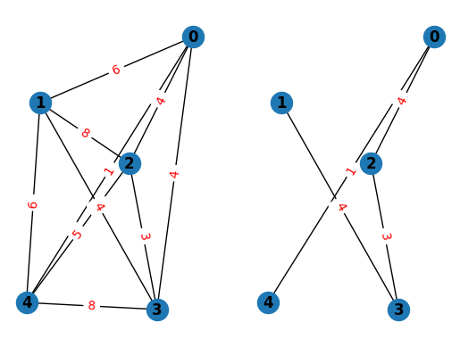
As expected, we have obtained the minimum spanning tree that satisfies the maximum degree constraint.

An advanced extension of the problem introduced here is the Steiner tree problem. In this problem, given edge costs \(c_{uv}\) and a subset of vertices \(U \subset V\), we seek a minimum-cost tree that contains every vertex in \(U\).

To solve the Steiner tree problem, one can use the same Hamiltonian as for the minimum spanning tree problem, but additional binary variables \(y_v\) are needed to indicate whether each vertex \(v \notin U\) is included in the tree.